Laplace transform works in the frequency domain, whereas initial conditions are for transient simulations in the time domain, so it does not make sense to apply an initial condition to a Laplace transform.
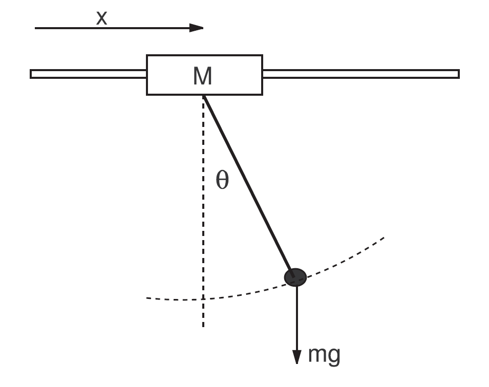
What does make sense is to do a time-domain simulation with the initial condition you mention. The fact that $u$ is equal to zero simply means that there are no external horizontal forces applied on the trolley. However, with an initial condition of 10° for $\theta$, the angular acceleration of mass will result in a non-zero $\theta$ as a function of time, which in turn will result in a non-zero $x$ as a function of time (c/f your first and second equations).
There are various tools out there for time-domain simulations, you may not need to use the Laplace transform at all for this, it's simply solving coupled differential equations. Here is an example with GNU Octave. I am using a state-space representation rather than a Laplace transform because it allows me better control of the states, which makes it easier to specify the initial conditions.
I define my state vector as:
$$
X = \begin{bmatrix} x \\ \dot{x} \\ \theta \\ \dot{\theta} \end{bmatrix}
$$
which gives:
$$
\dot{X} = \begin{bmatrix} \dot{x} \\ \ddot{x} \\ \dot{\theta} \\ \ddot{\theta} \end{bmatrix}
$$
The input is $u$ and output is $y$. The state-space representation is written as:
$$
\dot{X} = AX + Bu \\
y = CX + Du
$$
where $A$ is a 4x4 matrix, $B$ a 4x1 matrix, $C$ a 1x4 matrix and $D$ a 1x1 matrix, i.e. a scalar.
After re-arranging the differential equations to have $\dot{X}$ as a function of $X$ and $u$ only, I get the following matrices:
$$
A = \begin{bmatrix} 0 & 1 & 0 & 0 \\ 0 & -D/M & mg/M & 0 \\ 0 & 0 & 0 & 1 \\ 0 & D/(Ml) & -(g/l)*(1+m/M) & 0 \end{bmatrix} \\
B = \begin{bmatrix} 0 \\ 1/M \\ 0 \\ -1/(Ml) \end{bmatrix} \\
C = \begin{bmatrix} 1 & 0 & l & 0 \end{bmatrix} \\
D = 0
$$
In Octave, with some randomly chosen values, the code looks something like this
% Parameters
M=1;
m=0.15;
D=0.5;
g=9.81;
l=1;
theta_0=10*pi/180;

% State-space matrices
A = [0 1 0 0; 0 -D/M m*g/M 0; 0 0 0 1; 0 D/(M*l) -(g/l)*(1+m/M) 0];
B = [0 1/M 0 -1/(M*l)]';
C = [1 0 l 0];
DD = 0; % using DD to avoid confusion with parameter D
G = ss(A,B,C,DD);

% Time-domain simulation
t = linspace(0,10,500); % time vector
u = zeros(size(t));     % input vector u
x0 = [0 0 theta_0 0];   % initial conditions
lsim(G,u,t,x0)
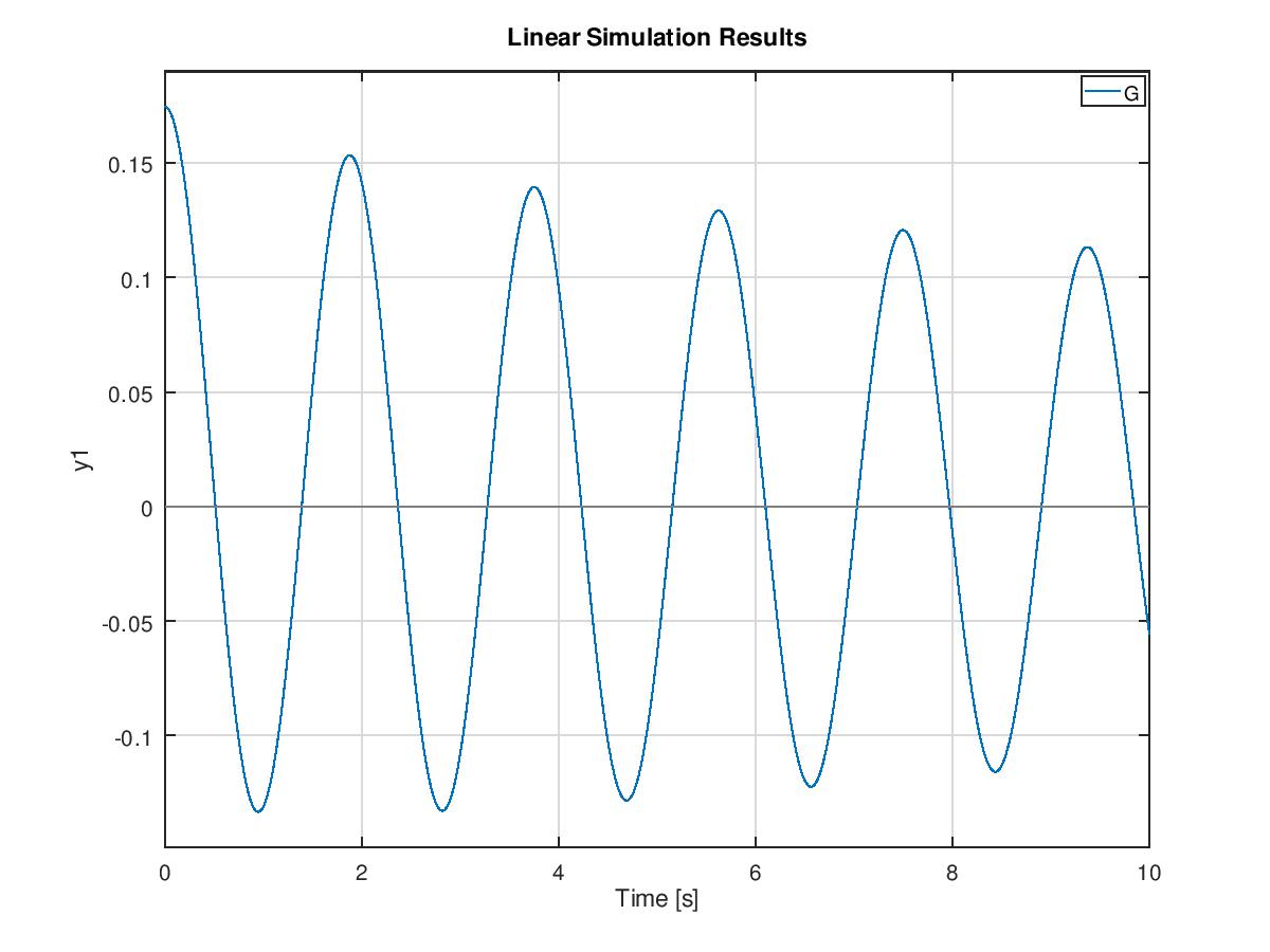
Which gives the following result:

The other method is to solve the differential directly with an ode solver, which yields the same results.
First you need to define a function to implement your differential equations:
function dx = gantry_crane(t,x)

  M = 1;
  m = 0.15;
  D = 0.5;
  l = 1;
  g = 9.81;

  dx(1) = x(2); % dx/dt
  dx(2) = (m*g*x(3) - D*dx(1))/M; %d^2x/dt^2
  dx(3) = x(4); % dtheta/dt
  dx(4) = -(m*g*x(3)+m*dx(2))/(m*l); %d^2theta/dt^2

 end
This is saved under the file name gantry_crane.m. You then call the ode solver as follows:
theta_0=10*pi/180;
x0 = [0 0 theta_0 0]
[t,x] = ode45(@gantry_crane,[0 10],x0);
y = x(:,1) + x(:,3); % y = x + l*theta and l=1
plot(t,y)
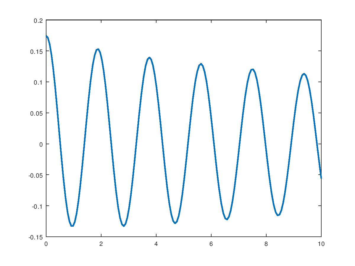
which gives the following result:
