I am stepping in the coding of motion simulation and have found in internet following python codes for practice purpose.
# Simulation of Mass-Spring-Damper System
import numpy as np
import matplotlib.pyplot as plt
# Model Parameters
c = 4 # Damping constant
k = 2 # Stiffness of the spring
m = 20 # Mass
F = 5 # Force
# Simulation Parameters
Ts = 0.1
Tstart = 0
Tstop = 60
N = int((Tstop-Tstart)/Ts) # Simulation length
x1 = np.zeros(N+2)
x2 = np.zeros(N+2)
x1[0] = 0 # Initial Position
x2[0] = 0 # Initial Speed
a11 = 1
a12 = Ts
a21 = -(Ts*k)/m
a22 = 1 - (Ts*c)/m
b1 = 0
b2 = Ts/m
# Simulation
for k in range(N+1):
    x1[k+1] = a11 * x1[k] + a12 * x2[k] + b1 * F
    x2[k+1] = a21 * x1[k] + a22 * x2[k] + b2 * F

# Plot the Simulation Results
t = np.arange(Tstart,Tstop+2*Ts,Ts)
#plt.plot(t, x1, t, x2)
plt.plot(t,x1)
plt.plot(t,x2)
plt.title('Simulation of Mass-Spring-Damper System')
plt.xlabel('t [s]')
plt.ylabel('x(t)')
plt.grid()
plt.legend(["x1", "x2"])
plt.show()
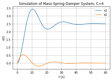
with the output plot
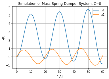
- By setting the damping coefficient C=0, I expected the amplitudes of the object's oscillation curve stays unchanged. But the curve shows increased amplitude over time. Does anyone know why the undamped object (C=0) has the oscillation with increased amplitude?
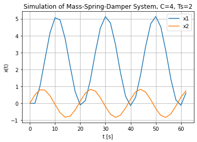
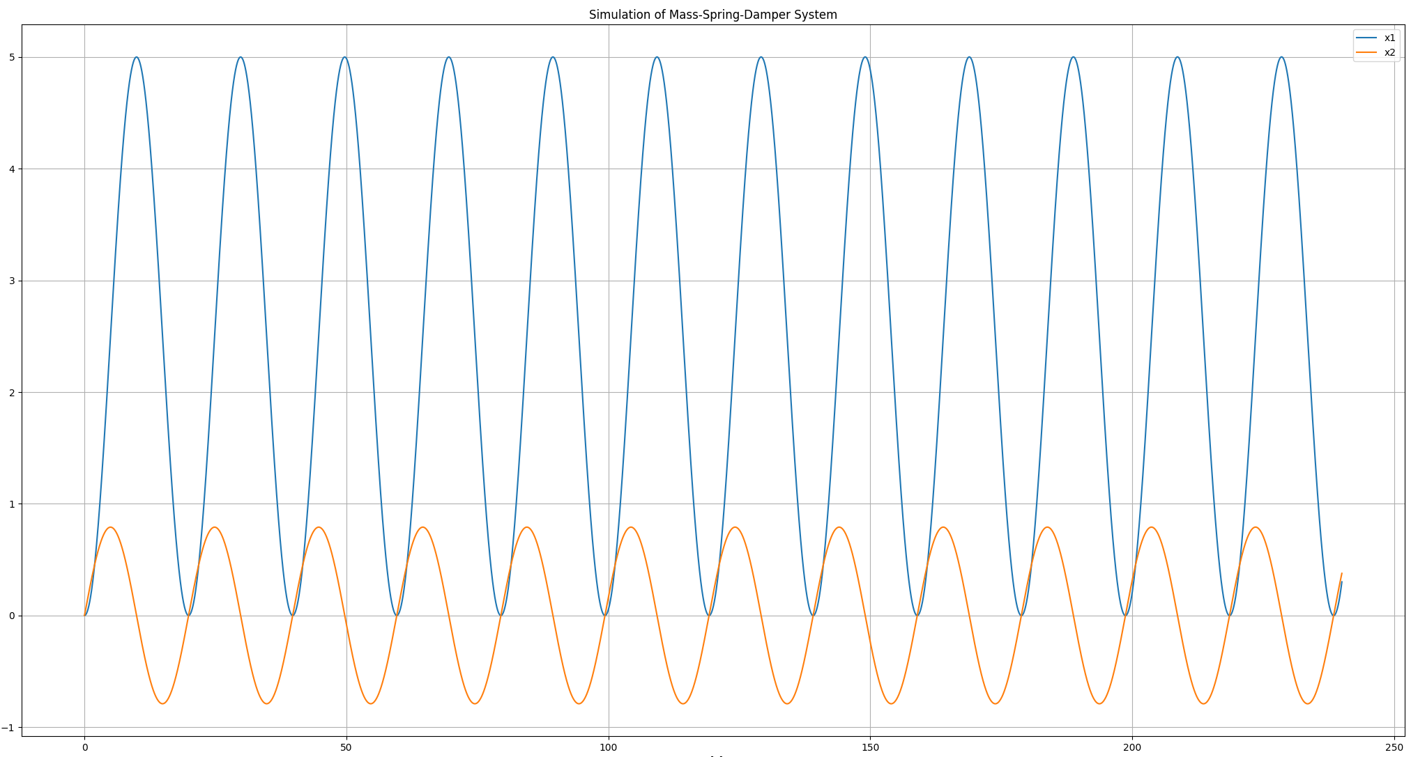
- The increment / time step seems to have influence on oscillation curve: by changing from 0.1 to 0.001 the curve shows slight change, while by increasing from 0.1 to 2 the curve becomes diverging (numerical instability - my assumption) Can anyone share your opinion/experiences herewith? Any rules/instructions for selecting the time step for reliable results?


