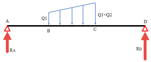
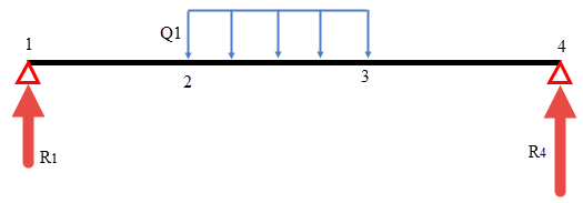
I found a better way to solve this problem by using singularity functions. Not only is the solution simple and elegant, one equation can be written for the entire beam! Also, the format for each equation is similar, so it is easy to copy the formula in a spreadsheet or program for one result (such as for the shear) and revise the equation for other results (such as the displacement) -- just change the multiplier and exponent. Furthermore, you do not need to calculate all of the variables (shear, moment, slope) to calculate any of the the other equations (such as displacement).
Not to go into too much detail, but singularity functions are like a switch to turn a load on. Furthermore, they can be integrated just like a normal equation. The singularity functions work as follow:
$$
\begin{align}
\langle x-a \rangle ^{-1} &=
\begin{cases}
0, & x \neq a \\
1, & x=a
\end{cases} \\
\langle x-a \rangle ^0 &=
\begin{cases}
0, & x \neq a \\
1, & x=a
\end{cases} \\
\text{if n>0, } \langle x-a \rangle ^n &=
\begin{cases}
0, & \text{x<a} \\
(x-a)^n, & \text{x>a}
\end{cases} \\
\end{align}
$$
$$
\begin{align}
& \int \langle x-a \rangle ^{-1} dx = \langle x-a \rangle ^0 \\
& \int \langle x-a \rangle ^0 dx = \langle x-a \rangle ^1 \\
& \int \langle x-a \rangle ^n dx = \frac{1}{n+1} \langle x-a \rangle ^{(n+1)}
\end{align}
$$
(https://www.colorado.edu/engineering/CAS/courses.d/Structures.d/IAST.Lect12.d/IAST.Lect12.pdf is a good example of using singularity functions to solve beam deflections.)
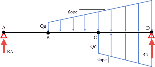
Using the singularity functions, the beam to solve

is represented as follows:

where $slope=(Q_C-Q_B)/(x_C-x_B)$, the load beginning with $Q_B$ continues for the remaining length, and the load beginning with $Q_C$ turns the load "off". (The singularity function turns a load on but not off, so any load that ends before the end of the beam requires a second load and singularity function to remove the load.)
Letting $x_A=0$ and $x_D=L$, the equation for the load $q(x)$ is $$
\bbox[yellow]
{
\begin{align}
q(x)=R_A\langle x \rangle ^{-1} + R_D\langle x-L \rangle ^{-1}&-Q_B\langle x-x_B \rangle ^0-slope\langle x-x_B \rangle ^1 \\
&+Q_C\langle x-x_C \rangle ^0+slope\langle x-x_C \rangle ^1
\end{align}
\tag 1
}
$$
The equation for the shear is $V(x)=\int q(x)dx$, $$
\bbox[yellow]
{
\begin{align}
V(x)=R_A\langle x \rangle ^{0} + R_D\langle x-L \rangle ^{0}&-Q_B\langle x-x_B \rangle ^1-\frac{1}{2}slope\langle x-x_B \rangle ^2 \\
&+Q_C\langle x-x_C \rangle ^1+\frac{1}{2}slope\langle x-x_C \rangle ^2
\end{align}
\tag 2
}
$$
The equation for the moment is $M(x)=\int V(x)dx$, $$
\bbox[yellow]
{
\begin{align}
M(x)=R_A\langle x \rangle ^{1} + R_D\langle x-L \rangle ^{1}&-\frac {1}{2}Q_B\langle x-x_B \rangle ^2-\frac{1}{6}slope\langle x-x_B \rangle ^3 \\
&+\frac {1}{2}Q_C\langle x-x_C \rangle ^2+\frac{1}{6}slope\langle x-x_C \rangle ^3
\end{align}
\tag 3
}
$$
From here on, singularity functions that begin at x=0 can be converted to regular functions, and singularity functions that begin at X=L can be dropped.
The equation for the slope is $EI\cdot\theta(x)=\int M(x)dx$, $$
\bbox[yellow]
{
\begin{align}
EI\cdot\theta(x)=\frac {1}{2}R_Ax^2+C_1 &-\frac {1}{6}Q_B\langle x-x_B \rangle ^3-\frac{1}{24}slope\langle x-x_B \rangle ^4 \\
&+\frac {1}{6}Q_C\langle x-x_C \rangle ^3+\frac{1}{24}slope\langle x-x_C \rangle ^4
\end{align}
\tag 4
}
$$
The equation for the deflection is $EI\cdot\delta(x)=\int \theta(x)dx$, $$
\bbox[yellow]
{
\begin{align}
EI\cdot\delta(x)=\frac {1}{6}R_Ax^3+C_1x+C_2 &-\frac {1}{24}Q_B\langle x-x_B \rangle ^4-\frac{1}{120}slope\langle x-x_B \rangle ^5 \\
&+\frac {1}{24}Q_C\langle x-x_C \rangle ^4+\frac{1}{120}slope\langle x-x_C \rangle ^5
\end{align}
\tag 5
}
$$
The reaction force $R_A$ can be determined from the moment equation. At x=L, M(x)=0,
\begin{align}
0=R_AL + R_D(0) &-\frac {1}{2}Q_B(L-x_B)^2-\frac{1}{6}slope(L-x_B)^3 \\
&+\frac {1}{2}Q_C(L-x_C)^2+\frac{1}{6}slope(L-x_C)^3\\
\tag 6
\end{align}
\begin{align}
R_AL =\frac {1}{6}[&+3Q_B(L-x_B)^2+slope(L-x_B)^3 \\
&-3Q_C(L-x_C)^2-slope(L-x_C)^3] \\
\tag 7
\end{align}
$$
\bbox[yellow]
{
\begin{align}
\text{thus }R_A =\frac {1}{6L}[&+3Q_B(L-x_B)^2+slope(L-x_B)^3 \\
&-3Q_C(L-x_C)^2-slope(L-x_C)^3]
\end{align}
\tag 8
}
$$
\begin{align}
\text{and }R_D &= \text{total load }-R_A \\
&= \frac 12(Q_B+Q_C)(x_C-x_B)-R_A
\tag 9
\end{align}
At x=0, $\delta=0$ from which $C_2=0$.
At x=L, $\delta=0$ from which $C_1$ is calculated as follows:
\begin{align}
EI\cdot(0)=\frac 16R_AL^3+C_1L &-\frac{1}{24}Q_B(L-x_B)^4-\frac{1}{120}slope(L-x_B)^5\\
&+\frac{1}{24}Q_C(L-x_C)^4+\frac{1}{120}slope(L-x_C)^5\\
\tag{10}
\end{align}
\begin{align}
-C_1L =\frac {1}{120}[20R_AL^3 &-5Q_B(L-x_B)^4- slope(L-x_B)^5\\
&+5Q_C(L-x_C)^4+slope(L-x_C)^5]\\
\tag{11}
\end{align}
$$
\bbox[yellow]
{
\begin{align}
\text{thus }C_1 =\frac {1}{120L}[-20R_AL^3 &+5Q_B(L-x_B)^4+ slope(L-x_B)^5\\
&-5Q_C(L-x_C)^4-slope(L-x_C)^5]\\
\end{align}
\tag{12}
}
$$
All values are now known, so any of the first 5 equations can be used to calculate the quantity at any position $x$ long the length of the beam $0<x<L$.
Some example results for $x_B=20,\, x_C=50,\, x_D=L=90,\, E=1\times10^6,\, I=8.5$:
\begin{array}{cc|cccc }
Q_B &Q_C &\theta_A &\theta_D &\delta_B &\delta_C \\
\hline
20 &35 &-0.0482 &+0.0429 &-0.8872 &-1.2971 \\
35 &10 &-0.0388 &+0.0325 &-0.7075 &-0.9958 \\
100 &-100 &+0.0036 &-0.0140 &+0.0987 &+0.3516
\end{array}


