edited body
Source Link

I have a high order discrete transfer function model which has the following form. When I use the allmargin function to get the gain margin, I get the following result:


G_uncoupled = tf(1,[0.25 0.5 0]);   
G_uncoupled_d = c2d(G_uncoupled,0.001,'zoh');     
D_d = tf([1 -1],[0.001 0],0.001);    
H_d = tf([(1 - exp(-10*2*pi*0.001)) 0],[1 -(exp(-10*2*pi*0.001))],0.001);   
delay_d = tf(1,[1 0],0.001);   

L_uncoupled = (G_uncoupled_d*delay_d^3)/(1 + G_uncoupled_d*D_d*H_d^n*B*delay_d^3G_uncoupled_d*D_d*H_d^1*1*delay_d^3);    


marginInfo = allmargin(L_uncoupled);

marginInfo = 

  struct with fields:

     GainMargin: [336.0257 9.8081e+05]
    GMFrequency: [37.5848 1.7955e+03]
    PhaseMargin: [90.0569 84.1254]
    PMFrequency: [0.0019 0.6617]
    DelayMargin: [8.2179e+05 2.2191e+03]
    DMFrequency: [0.0019 0.6617]
         Stable: 0

When I plot the bode plot of this transfer function, I get the following graph, from the graph I can see two phase margins, but I only see a gain margin 336.0257(50.5dB) at 37.5 rad. For the second frequency 1.7955e+03, I can't see the gain margin at this frequency from the Bode plot, how did MATLAB get this value or what does this value represent?
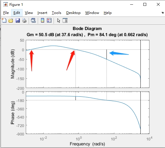
enter image description here

I have a high order discrete transfer function model which has the following form. When I use the allmargin function to get the gain margin, I get the following result:


G_uncoupled = tf(1,[0.25 0.5 0]);   
G_uncoupled_d = c2d(G_uncoupled,0.001,'zoh');     
D_d = tf([1 -1],[0.001 0],0.001);    
H_d = tf([(1 - exp(-10*2*pi*0.001)) 0],[1 -(exp(-10*2*pi*0.001))],0.001);   
delay_d = tf(1,[1 0],0.001);   

L_uncoupled = (G_uncoupled_d*delay_d^3)/(1 + G_uncoupled_d*D_d*H_d^n*B*delay_d^3);    


marginInfo = allmargin(L_uncoupled);

marginInfo = 

  struct with fields:

     GainMargin: [336.0257 9.8081e+05]
    GMFrequency: [37.5848 1.7955e+03]
    PhaseMargin: [90.0569 84.1254]
    PMFrequency: [0.0019 0.6617]
    DelayMargin: [8.2179e+05 2.2191e+03]
    DMFrequency: [0.0019 0.6617]
         Stable: 0

When I plot the bode plot of this transfer function, I get the following graph, from the graph I can see two phase margins, but I only see a gain margin at 37.5 rad. For the second frequency 1.7955e+03, I can't see the gain margin at this frequency from the Bode plot, how did MATLAB get this value or what does this value represent?

enter image description here

I have a high order discrete transfer function model which has the following form. When I use the allmargin function to get the gain margin, I get the following result:


G_uncoupled = tf(1,[0.25 0.5 0]);   
G_uncoupled_d = c2d(G_uncoupled,0.001,'zoh');     
D_d = tf([1 -1],[0.001 0],0.001);    
H_d = tf([(1 - exp(-10*2*pi*0.001)) 0],[1 -(exp(-10*2*pi*0.001))],0.001);   
delay_d = tf(1,[1 0],0.001);   

L_uncoupled = (G_uncoupled_d*delay_d^3)/(1 + G_uncoupled_d*D_d*H_d^1*1*delay_d^3);    


marginInfo = allmargin(L_uncoupled);

marginInfo = 

  struct with fields:

     GainMargin: [336.0257 9.8081e+05]
    GMFrequency: [37.5848 1.7955e+03]
    PhaseMargin: [90.0569 84.1254]
    PMFrequency: [0.0019 0.6617]
    DelayMargin: [8.2179e+05 2.2191e+03]
    DMFrequency: [0.0019 0.6617]
         Stable: 0

When I plot the bode plot of this transfer function, I get the following graph, from the graph I can see two phase margins, but I only see a gain margin 336.0257(50.5dB) at 37.5 rad. For the second frequency 1.7955e+03, I can't see the gain margin at this frequency from the Bode plot, how did MATLAB get this value or what does this value represent?

enter image description here

Source Link

MATLAB allmargin() function return multiple GainMargin, but how to identify them on the Bode plot?

I have a high order discrete transfer function model which has the following form. When I use the allmargin function to get the gain margin, I get the following result:


G_uncoupled = tf(1,[0.25 0.5 0]);   
G_uncoupled_d = c2d(G_uncoupled,0.001,'zoh');     
D_d = tf([1 -1],[0.001 0],0.001);    
H_d = tf([(1 - exp(-10*2*pi*0.001)) 0],[1 -(exp(-10*2*pi*0.001))],0.001);   
delay_d = tf(1,[1 0],0.001);   

L_uncoupled = (G_uncoupled_d*delay_d^3)/(1 + G_uncoupled_d*D_d*H_d^n*B*delay_d^3);    


marginInfo = allmargin(L_uncoupled);

marginInfo = 

  struct with fields:

     GainMargin: [336.0257 9.8081e+05]
    GMFrequency: [37.5848 1.7955e+03]
    PhaseMargin: [90.0569 84.1254]
    PMFrequency: [0.0019 0.6617]
    DelayMargin: [8.2179e+05 2.2191e+03]
    DMFrequency: [0.0019 0.6617]
         Stable: 0

When I plot the bode plot of this transfer function, I get the following graph, from the graph I can see two phase margins, but I only see a gain margin at 37.5 rad. For the second frequency 1.7955e+03, I can't see the gain margin at this frequency from the Bode plot, how did MATLAB get this value or what does this value represent?

enter image description here