Related - how do i calculate an estimate for the properties of a composite material
The reference to Mil Handbook 17F, p. 213 is summarized here:

Computation of effective elastic moduli is a very difficult problem in
elasticity theory and only a few simple models permit exact analysis.
One type of model consists of periodic arrays of identical circular fibers, e.g., square periodic arrays or hexagonal periodic arrays ... These models are analyzed by numerical finite difference or finite element procedures. Note that the square array is not a suitable model for the majority of Uni-Directional Composites since it is not transversely isotropic.
The composite cylinder assemblage (CCA) model permits exact analytical determination of effective elastic moduli ... Consider a collection of composite cylinders, each with a circular fiber core and a concentric matrix shell. The size of the cylinders may vary but the ratio of core radius to shell radius is held constant. Then...

(Where $V_f$ is the volume fraction of fibers to the total amount of material.
$X_{m}$ is a property of the matrix, $X_{f}$ is a property of the fiber, and $E, G, k$ are the elastic modulus, shear modulus, and bulk modulus properties. The bulk modulus, k, can be computed for isotropic materials as $\frac{E}{2(1-\nu-2\nu^2)}$, where $\nu$ is the Poisson's ratio. The G without a subscript is a typo, and should be replaced with $G_m$)
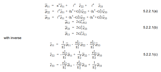
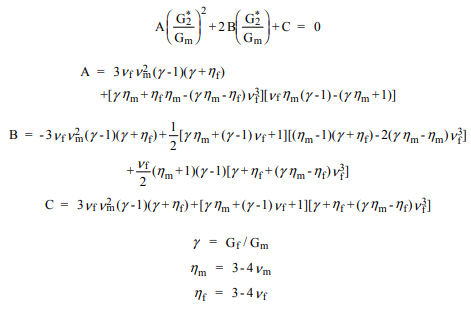
A preferred alternative is to use a method of approximation which has been called the Generalized Self Consistent Scheme (GSCS). According to this method, the stress and strain in any fiber is approximated by embedding a composite cylinder in the effective fiber composite material. The volume fractions of fiber and matrix in the composite cylinder are those of the entire composite. Such an analysis ... results in a quadratic equation for the shear modulus...

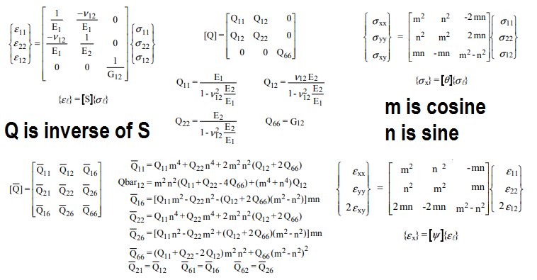
The net algorithm is to compute the effective bulk modulus $k^*$, 12 poisson's ratio $\nu_{12}^*$, and young's modulus $E_{1}^*$ first, then use the quadratic formula listed to calculate the second shear modulus, $G_2^*$. Using $G_2^*$, $E_2^*$, $\nu_{23}^*$, and $G_1$ can be calculated. These are in the local coordinate system of the fiber. To translate to global coordinates:

We can then rotate the fiber to find the properties of the uni-directional composite to find the properties in an arbitrary direction:

where Qbar is the rotated matrix, and Q is the original inverse matrix. For a stochastic model, the angle of the fiber and the volume fraction can be the inputs, and the outputs would be the resulting properties. Note that for a uniform random distribution, it is possible to integrate the Qbar matrix as theta varies from 0 to $2\pi$, then divide by $2\pi$ to obtain a symmetrical matrix. The results from this method match well with data on random fiber materials in the fiberglass industry.
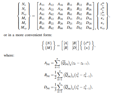
As you asked about a differential equation, we'd need to review the appropriate theory from this point on. For example, the classical plate equation, $$\nabla^2\nabla^2 = \frac{q}{D}$$, works partly. We have to include another stoichastic variable, the height of the fiber inside of a block of concrete. The closer the fiber is to the top, the stiffer the block will be against the bending load. The block can be divided into arbitrary segments of uniform thickness, and the volume of the fibers in each segment is added, generating different Qbars. A different distribution would result in different properties of the block:

This matrix, called the ABD matrix, would then redefine the plate equation as follows:
$$D_{11}\frac{\partial^4 w}{\partial x^4} + 2(D_{12}+2 D_{66})\frac{\partial^4 w}{\partial x^2 \partial y^2} + D_{22}\frac{\partial^4 w}{\partial y^4} = q(x,y)$$
for the simplest of cases (B matrix irrelevant, no transverse loading, etc...). The cases go stranger from there, but can be derived from the original derivations, but stopping when the model says to assume the stress is proportional to the stain.
