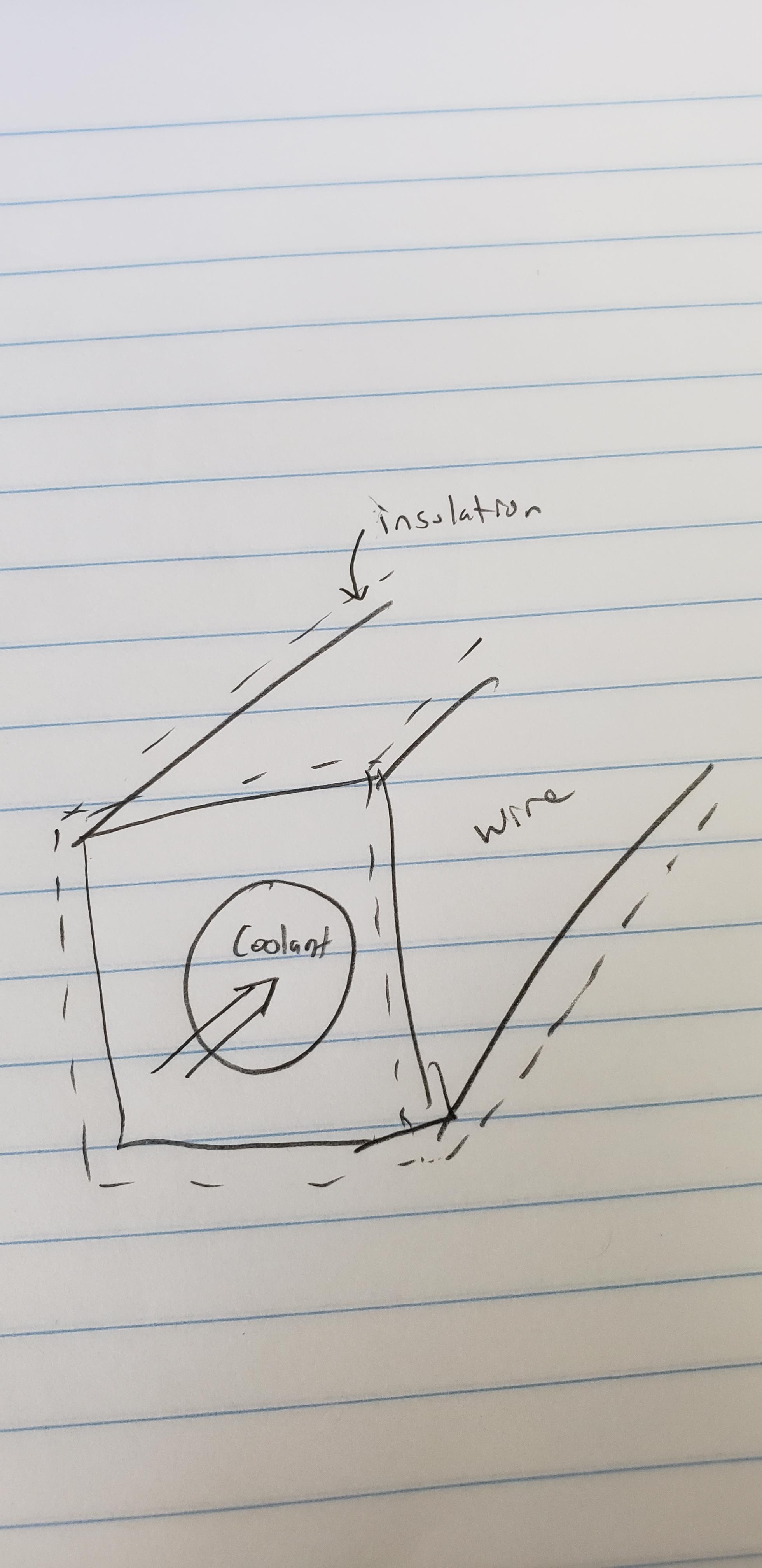
Foundations
The heat transfer problem has three considerations. First is steady state versus unsteady state. The former case is far easier and is all that I will consider here. Second is the temperature profiles axial in $z$ and radial in $r$. The best approach is to presume that separation of variables will work. Finally, the last consideration is the influence of heat transfer internally and externally to the cylinder while generating uniform power in the shell $P = i^2R$.
Also, for simplicity, neglect the (electrical) insulation layer on the outside of the wire.
The starting point is to build each of the cases one step at a time.
Axial versus Radial Gradients - Biot Number Estimates
In the ideal case, we allow for separation of variables to make $T(r,z) = Tr(r)Tz(z)$. A starting point for this is to determine the effective Biot numbers for radial heat transfer.
$$Bi_{rw} = h_w \Delta R/k \hspace{1cm} Bi_{ra} = h_a \Delta R/k $$
In these, $h_w, h_a$ are the convection coefficients of the flowing water or surrounding air, $\Delta R$ is the outer minus inner radius $\Delta R = r_o - r_i$, and $k$ is the thermal conductivity of the wire. When $Bi < 0.1$, the wire functions in a lumped analysis. The radial gradients can be neglected.
Axial Gradients Only
Water Cooling Only
Consider the system for the case that $Bi_{rw} < 0.1$ with perfect thermal insulation around the wire. This will give the maximum temperature that can be expected in the wire. The energy balance along the flow says that total power input $P$ must be taken out by the flowing fluid (water) with mass flow $\dot{m}$ and specific heat $\tilde{C}_p$. The fluid temperature changes from input $T_{wi}$ to output $T_{wf}$.
$$ \dot{m}\tilde{C}_p(T_{wf,max} - T_{wi}) = P$$
The subscript "max" indicates the case of maximum output temperature on the fluid. You can also use this to establish that, in this case, the temperature profile in the fluid is linear along the axis.
$$ \dot{m}\tilde{C}_p(T_w(z) - T_{wi}) = P \frac{z}{L}$$
or
$$ T_w(z) - T_{wi} = P\left(\frac{z}{L}\right)\left(\frac{1}{\dot{m}\tilde{C}_p}\right)$$
The differential energy balance on the wire with no radial gradients and with the external wall as a perfect thermal insulator is as below with $r_i$ as the radius of the channel.
$$ h_w 2\pi r_i\left(T_z(z) - T_w(z)\right) dz = P \frac{dz}{L}$$
This gives the temperature in the wire as below with $A_i$ as the area of the water channel.
$$ T_w(z) - T_{wi} = P \left(\frac{z}{L}\right)\left(\frac{1}{\dot{m}\tilde{C}_p} + \frac{1}{h_w A_i}\right)$$
Including External Convection to Air
When we add convection to air, the energy balance to the internal fluid (water) written in differential form is as below with $r_o$ as the external radius of the wire and $T_a$ as the air temperature.
$$ \dot{m}\tilde{C}_p dT_w + h_a 2\pi r_o (T_z(z) - T_a) dz = P \frac{dz}{L}$$
The differential energy balance on the wire at any axial position $z$ is the equation below with $r_i$ as the channel radius.
$$ h_w 2\pi r_i(T_z(z) - T_w(z))dz + h_a 2\pi r_o(T_z(z) - T_a)dz = P \frac{dz}{L}$$
These are two coupled differential equations to solve for $T_w(z)$ and $T_z(z)$. In all cases, the water and wire temperatures will be lower than the case for water cooling only because a portion of the power generation is now removed by the air.
Radial Gradients
The radial gradient problem is easily solved for a hollow cylinder with fixed internal and external wall temperatures $T_{ci}$ and $T_{co}$. The steady state profiles are well-documented in textbooks on heat transfer (see Chapter 17 in Welty, et.al). At any position $z$, the radial temperature profile will have the form below.
$$ \frac{T_r - T_{co}}{T_{ci} - T_{co}} = \frac{\ln(r/r_o)}{\ln(r_i/r_o)} $$
Following the format of separation of variables, the radial gradient is superimposed on the axial profile from above.
The link between the wall temperatures $T_{ci}, T_{co}$ and the water or air temperatures occurs as convection. This is an entirely separate issue to tackle. It can only be done once a proof is established that separation of variables is valid.
Unsteady State
This level of analysis is best done step-wise. Include time on the axial profile with insulated boundary, then include time on the axial profile including air convection, and finally consider time only on the radial boundary.
