System Dynamics Modeling

Question

I am trying to model this system but am having difficulties in setting up the equations of motion. This is a simplified model of a motorcycle suspension system, where P is the ground in the image below. In addition, the variable $u$ is the input to the system, which is the displacement from the ground (like a motorcycle going over a bump).

Consider mass $m_2$ first. Keeping $m_1$ fixed and displacing $m_2$ a bit yields the equation of motion for $m_2$ as $$ m_2 \ddot{y} = -k_2 (y-x) -b_2 (\dot{y} - \dot{x}) $$

And similarly, for $m_1$, keeping $m_2$ and $u$ fixed and displacing $m_1$ a little bit, the equation of motion comes out to be $$ m_1 \ddot{x} = -k_1 (x-u) -b_1(\dot{x} - \dot{u}) - k_2(x-y) - b_2(\dot{x}-\dot{y}) $$

The first two term on the RHS come from the coupling of $x$ with $u$ while the second and third come from the coupling of $m_1$ and $m_2$, or equivalently from Newton's third law. However, the textbook solution only has the first two terms, and not the interaction between $m_1$ and $m_2$ for the EOM of mass 1. I am extremely confused as to why this is the case. Is it because they are vertical and not horizontal? How would the EOM change if the scenario was all horizontal?

Answer 1

Deriving the system dynamics is systematically done using free-body diagrams, one diagram per body:

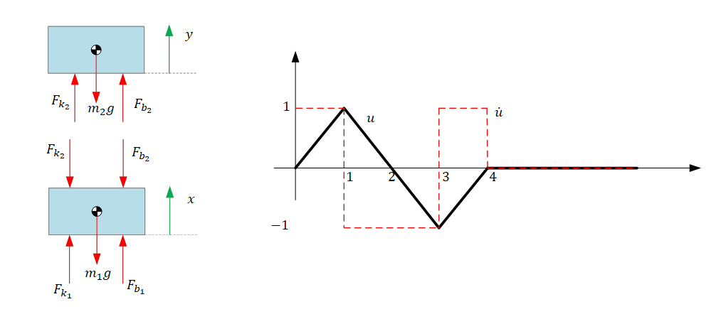
The sign of spring and damper forces are easily determined by considering the motion of one state variable at a time. For example, the spring $k_2$ will push on the mass $m_2$ if $x>0$ while $y$ is held fixed and it will pull on the mass $m_2$ if $y>0$ while $x$ is held fixed.
Hence, relative to $m_2$, that spring force will be $F_{k_2}=k_2(x-y)$ in the positive $y$-direction.
Furthermore, all force elements that connects two bodies, acting in a given direction on one body, will act with equal magnitude in the opposite direction on the other body.

The equations of motion can be written $$\begin{align}m_1\ddot{x}&=F_{k_1}+F_{b_1}-F_{k_2}-F_{b_2}-m_1g\\ &=k_1(u-x)+b_1(\dot{u}-\dot{x})-k_2(x-y)-b_2(\dot{x}-\dot{y})-m_1g\\ \\ m_2\ddot{y}&=F_{k_2}+F_{b_2}-m_2g\\ &=k_2(x-y)+b_2(\dot{x}-\dot{y})-m_2g \end{align}$$ In state-space form, using state vector, $\mathbf{x}=\begin{bmatrix}x&y&\dot{x}&\dot{y}\end{bmatrix}^T$ and input vector, $\mathbf{u}=\begin{bmatrix}u&\dot{u}\end{bmatrix}^T$ we get the system $$\dot{\mathbf{x}}=\displaystyle\begin{bmatrix}0&0&1&0 \\ 0&0&0&1 \\ \displaystyle-\frac{(k_1+k_2)}{m_1}&\displaystyle\frac{k_2}{m_1}&\displaystyle-\frac{(b_1+b_2)}{m_1}&\displaystyle\frac{b_2}{m_2}\\ \displaystyle\frac{k_2}{m_2}&\displaystyle-\frac{k_2}{m_2}&\displaystyle\frac{b_2}{m_2}&\displaystyle-\frac{b_2}{m_2}\end{bmatrix}\mathbf{x}+\begin{bmatrix} 0&0\\0&0\\\displaystyle\frac{k_1}{m_1}&\displaystyle\frac{b_1}{m_1}\\0&0\end{bmatrix}\mathbf{u}+\begin{bmatrix}0\\0\\-g\\-g\end{bmatrix}$$ If we neglect gravity we get the standard form: $$\dot{\mathbf{x}}=\mathbf{A}\mathbf{x}+\mathbf{B}\mathbf{u}$$ 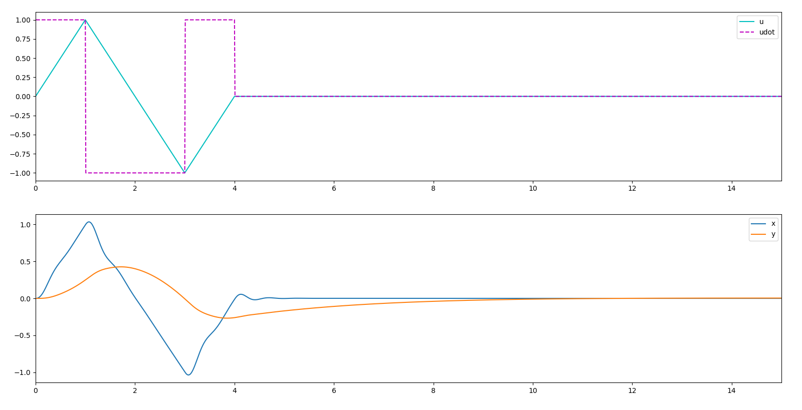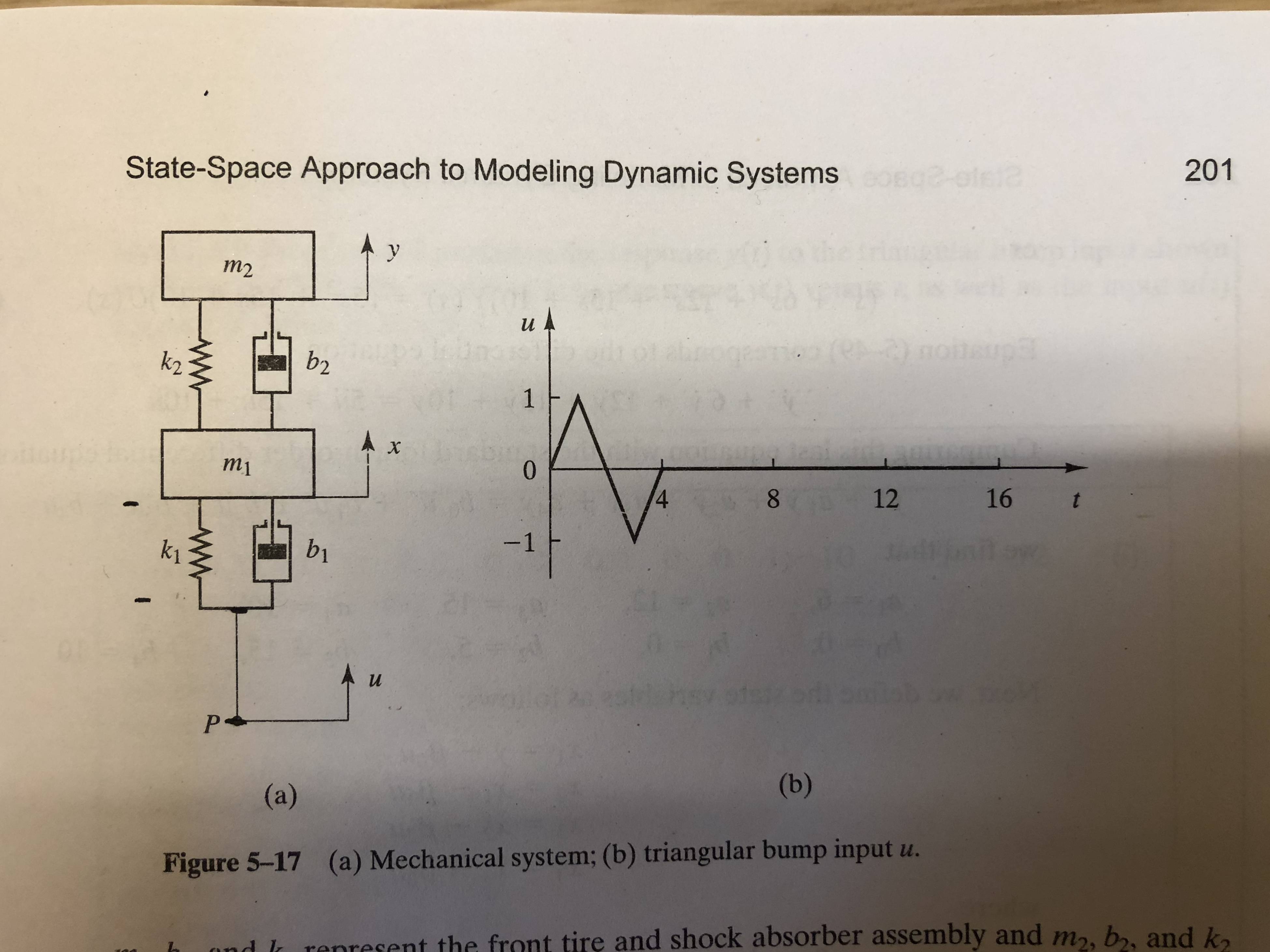The road-elevation input $u$ can be interpreted as the integral of a composite step function $\dot{u}$, where $$\dot{u}=\begin{cases} 1 && t\in[0,1) \\ -1 && t\in[1,3)\\ 1 && t\in[3,4) \\ 0 && t \geq 4\end{cases}$$ We can test the model quickly as follows, using forward Euler integration with NumPy and Python

import numpy as np
import matplotlib.pyplot as plt

# Mass, spring and damper constants
m1,m2,k1,k2,b1,b2 = 15,100,2000,10,60,60

# Integration scheme and initial values
h = 0.01
N = int(15/h)
t = np.linspace(h,15,N)
x = np.array([[0,0,0,0]]).T

# Input signals
udot = 1 * (t <= 1) - 1 * (t > 1) + 2 * (t > 3) - 1 * (t > 4)
u = np.cumsum(udot)*h

# System matrices
A = np.array([
    [0, 0, 1, 0],
    [0, 0, 0, 1],
    [-(k1+k2)/m1, k2/m1, -(b1+b2)/m1, b2/m1],
    [k2/m2, -k2/m2, b2/m2, -b2/m2]
])
B = np.array([
    [0, 0],
    [0, 0],
    [k1/m1, b1/m1],
    [0, 0]
])

# Book-keeping lists
xs = []
ys = []

for i in range(0,N):

    xdot = A @ x + B @ np.array([[u[i]], [udot[i]]])
    x = x + xdot*h
    xs.append(x[0,0])
    ys.append(x[1,0])

fig = plt.figure()
ax1 = fig.add_subplot(211)
ax1.plot(t, u, 'c', t, udot, 'm--')
plt.xlim([0,15])
plt.legend(['u','udot'])
ax2 = fig.add_subplot(212)
ax2.plot(t, xs, t, ys)
plt.xlim([0,15])
plt.legend(['x','y'])

Answer 2

You're equations of motion are correct. Your book is either wrong, or is making the assumption that $m_1 \gg m_2$ in which case the terms contributing from the interaction with $m_2$ would be negligible.