Modeling Transient Heat Transfer between two 1-D materials

Question

I have been working on creating a 1-D model of a material with a layer of heat resistant material stuck to it. For this I have been trying to use the implicit finite-differential method. The equations are as follows:

$$ \dot{E}_{in} - \dot{E}_{out} = \dot{E}_{st} $$ or $$ \frac{1}{\alpha} \frac{dT}{dt}= \frac{d^2T}{dx^2} $$ Where $\alpha = \frac{k}{\rho C_p} $

So, if there is only one material, an internal node equation would look like (I am assuming all flow in into the node for sign convention, n is the node location, p is the time step, and x is the thickness of a node): $$ \frac{k A}{\Delta x}(T^{p+1}_{n+1}-T^{p+1}_{n}) + \frac{k A}{\Delta x}(T^{p+1}_{n-1}-T^{p+1}_{n}) = \frac{C_p \rho A \Delta x }{\Delta t}(T^{p+1}_{n}-T^{p}_{n}) $$ or $$ (1+2*Fo)T^{p+1}_n - Fo(T^{p+1}_{n-1}+T^{p+1}_{n+1}) = T^p_n $$ Where, $Fo = \frac{\alpha \Delta t}{(\Delta x)^2}$

The surface node equation looks like: $$ {h A}(T_\infty-T^{p+1}_{n}) + \frac{k*A}{\Delta x}(T^{p+1}_{n-1}-T^{p+1}_{n}) = \frac{C_p \rho A \Delta x }{2 \Delta t}(T^{p+1}_{n}-T^{p}_{n}) $$ or $$ (1+2Fo + 2FoBi)T^{p+1}_n-2Fo(T^{p+1}_{n-1}+BiT_\infty) = T^p_n $$ Where, $Bi = \frac{h\Delta x}{k}$

This seems to work pretty good for me when I use just one material. I give it some initial conditions and run it to steady state then check it against a simple steady state resistance model and there is a match.

I begin to bump into issues when I put in an internal material boundary. This is the equation I was using to simulate it (This calculation is for a node in material A adjacent to a node in material B)

$$ \frac{(k_b +k_a )A}{\Delta x_b+\Delta x_a}(T^{p+1}_{n+1}-T^{p+1}_{n}) + \frac{k_a A}{\Delta x_a}(T^{p+1}_{n-1}-T^{p+1}_{n}) = \frac{C_{pa} \rho_a A \Delta x_a }{\Delta t}(T^{p+1}_{n}-T^{p}_{n}) $$ or $$ (1+ Fo + Fo_{ab})T^{p+1}_n-FoT^{p+1}_{n-1}-Fo_{ab}T^{p+1}_{n+1} = T^p_n $$ Where, $Fo_{ab} = \frac{\alpha_{ab} \Delta t}{\Delta x_a(\Delta x_b+\Delta x_a)}$ and $\alpha_{ab} = \frac{k_b+k_a}{\rho_a C_{pa}} $ Note: if the materials are the same $Fo_{ab} = Fo$ this equation becomes a same as the boundary equation above.

With this boundary added I again created a steady-state resistive model to check against and found about a 10% difference, which was not expected. (note:updated to add in an averaging of k values to remove this difference, not sure if its right, but it fixed the error) Below is a diagram showing the two model setups:

For the test case, I used the arbitrary constants: $$\Delta t = 0.15$$ $$Nodes_a = Nodes_b = 5$$ Note, number of nodes is different than in the picture above (4). $$\Delta x_a = \Delta x_b = Length/(Nodes-0.5) = 10/4.5 = 2.2222$$ $$h_a = h_b = 1$$ $$\rho_a = \rho_b = 1$$ $$C_{pa} = C_{pb} = 1$$ $$k_a = 5$$ $$k_b = 10$$

Should I be getting this 10% difference between the two models? (updated to fix difference, still not sure if the new equation is correct though) Is this equation I am using for the material boundary correct?

Btw, many of the equations for surface nodes and boundary nodes came from the book: "Fundamentals of Heat and Mass Transfer" by Incropera and DeWitt.5th edition, section 5.9.2.

Answer 1

I am guessing, you are solving the following system:

$$\partial_t T = \alpha_i \partial_x^2 T$$

with $\alpha_i=\kappa_i/\rho_i c_{p,i}$ for material $i$, subject to the conditions:

$$T\left(x,0\right)=T_\infty\quad T\left(0,t\right) = T_h \quad -\kappa\partial_xT\left(L,t\right)=h\left[T\left(L,t\right)-T_\infty\right]$$

Now you can approach simulating different materials in the following way:

1. Define an interface at a node at $x_b$; make $\alpha_i$ a function of $x$, have $\alpha=\alpha_1$ in region $0 \le x \le x_b$ and $\alpha=\alpha_2$ in region $x_b \le x \le L$.
2. Impose thermal equilibrium and heat flux continuity at the interface; i.e.: $$T\left(x_b^-\right)=T\left(x_b^+\right)\quad -\kappa_1\partial_xT\left(x_b^-\right)=-\kappa_2\partial_xT\left(x_b^+\right)$$

I would make the node corresponding to $x=0$ equal to $T=T_h$ and the node corresponding to $x=L$ equal to:

$$-\kappa_2\frac{T\left(L^-,t\right)-T\left(L,t\right)}{\Delta x}=h\left[T\left(L,t\right)-T_\infty\right]$$ $$T\left(L,t\right)=\frac{T\left(L^-,t\right)-\beta T_\infty}{1-\beta} \quad \beta=\frac{h\Delta x}{\kappa_2}$$

where $T\left(L^-,t\right)$ is the node to the left of $x=L$.

Solution based on Finite Volume

I decided to take another look at this and came up with a solution based on Finite Volume which I think works better. Coincidentally, a 1D FV solution is the same as a 1D FD solution except the grid is staggered. Let's start simple and add complexity after everything is working correctly.

Some important assumptions i have made in the analysis:

• Nodes are monospaced at $\Delta x=L/N$ where $L$ is the length of the domain and $N$ the number of nodes; this simplifies the analysis considerably.
• The boundaries and interface are located exactly halfway between nodes, this allows a second order accurate approximation of temperatures and gradients at those boundaries.
• I do not bother with the time integration of these systems, i leave that up to a relevant ODE solver which can handle linear systems (see usage of odeint solver provided by Scipy in the Python code appended below). A good solver has adaptive time stepping allowing me to avoid any issues with numerical instability related to the CFL criterium.

We start with simple diffusion between two boundaries defined by the system: $$\partial_{t}T=\alpha\partial_{x}^{2}T$$ $$T\left(x,0\right)=T_{\infty}\quad T\left(0,t\right)=T_{h}\quad T\left(L,t\right)=T_{\infty}$$

In FV we define an average temperature over the control volume $dV=Adx$: $$\bar{T}_{i}=\frac{\int_{V}TdV}{\int_{V}dV}=\frac{1}{\Delta x}\int_{i-\frac{1}{2}\Delta x}^{i+\frac{1}{2}\Delta x}Tdx$$

We then integrate our PDE: $$\frac{1}{\Delta x}\int_{i-\frac{1}{2}\Delta x}^{i+\frac{1}{2}\Delta x}\partial_{t}Tdx=\frac{\alpha}{\Delta x}\int_{i-\frac{1}{2}\Delta x}^{i+\frac{1}{2}\Delta x}\partial_{x}^{2}Tdx$$

$$\partial_{t}\bar{T}_{i}=\frac{\alpha}{\Delta x}\left[\left.\partial_{x}T\right|_{i-\frac{1}{2}\Delta x}-\left.\partial_{x}T\right|_{i+\frac{1}{2}\Delta x}\right]$$

$$\partial_{t}\bar{T}_{i}=\frac{\alpha}{\Delta x^{2}}\left[\bar{T}_{i-\Delta x}-2\bar{T}_{i}+\bar{T}_{i+\Delta x}\right]$$

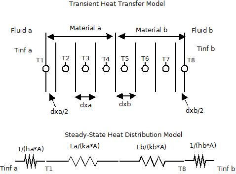
Here $0 \le i \le N-1$ are the inclusive nodes, i.e. the nodes lie within the domain, according to this schematic:

The conversion from node position to spatial position is given by:

$$i=N\frac{x}{L}-\frac{1}{2}$$

In this staggered grid, the boundaries $x=0$ and $x=L$ are located halfway between two nodes. However, if we imagine a ghost node at $i=-1$ and $i=N$, we can define the boundary temperatures as: $$T_{h}=\frac{\bar{T}_{-1}+\bar{T}_{0}}{2}\rightarrow\bar{T}_{-1}=2T_{h}-\bar{T}_{0}$$

$$T_{\infty}=\frac{\bar{T}_{N-1}+\bar{T}_{N}}{2}\rightarrow\bar{T}_{N}=2T_{\infty}-\bar{T}_{N-1}$$

This then yields the following ODE's for $i=0$ and $i=N-1$: $$\partial_{t}\bar{T}_{0} = \frac{\alpha}{\Delta x^{2}}\left[\bar{T}_{-1}-2\bar{T}_{0}+\bar{T}_{1}\right] = \frac{\alpha}{\Delta x^{2}}\left[2T_{h}-3\bar{T}_{0}+\bar{T}_{1}\right]$$

$$\partial_{t}\bar{T}_{N-1} = \frac{\alpha}{\Delta x^{2}}\left[\bar{T}_{N-2}-2\bar{T}_{N-1}+\bar{T}_{N}\right] = \frac{\alpha}{\Delta x^{2}}\left[\bar{T}_{N-2}-3\bar{T}_{N-1}+2T_{\infty}\right]$$

Now we are in a position to define our linear system. If we define a temperature vector: $$\bar{\boldsymbol{T}}=\begin{bmatrix}\bar{T}_{0} & \bar{T}_{1} & \cdots & \bar{T}_{N-2} & \bar{T}_{N-1}\end{bmatrix}^{T}$$

the ODE system can be written as: $$\partial_{t}\bar{\boldsymbol{T}}=\omega\left(\boldsymbol{A}\cdot\bar{\boldsymbol{T}}+\boldsymbol{b}\right) \quad \omega = \frac{\alpha}{\Delta x^{2}}$$

where: $$\boldsymbol{A}=\begin{bmatrix}-3 & 1 & 0 & 0 & 0\\ 1 & -2 & 1 & 0 & 0\\ 0 & \ddots & \ddots & \ddots & 0\\ 0 & 0 & 1 & -2 & 1\\ 0 & 0 & 0 & 1 & -3 \end{bmatrix}\quad \boldsymbol{b}=\begin{bmatrix}2T_{h}\\ 0\\ 0\\ 0\\ 2T_{\infty} \end{bmatrix}$$

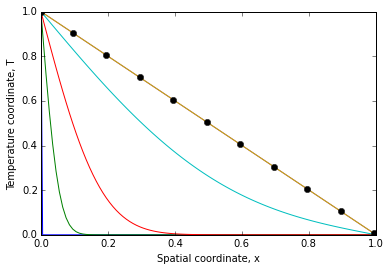
Solving this system for $T_h=1$, $T_{\infty}=0$, $L=1$, gives the following result:

$\hskip1in$

where the temperature profiles are given at different times and the markers are the analytical solution given by:

$$T=T_h-\left(T_h-T_{\infty}\right)\frac{x}{L}$$

Adding a convective boundary condition

Let's change the boundary condition at $x=L$ to:

$$-k\partial_{x}T\left(L,t\right)=h\left(T\left(L,t\right)-T_{\infty}\right)$$

We discretize this condition: $$-k\left(\frac{\bar{T}_{N}-\bar{T}_{N-1}}{\Delta x}\right)=h\left(\frac{\bar{T}_{N-1}+\bar{T}_{N}}{2}-T_{\infty}\right)$$

and rearrange for the ghost node temperature at $i=N$: $$\bar{T}_{N}=\frac{\mathrm{Nu}_{x}}{1+\frac{1}{2}\mathrm{Nu}_{x}}T_{\infty}+\frac{1-\frac{1}{2}\mathrm{Nu}_{x}}{1+\frac{1}{2}\mathrm{Nu}_{x}}\bar{T}_{N-1}\quad\mathrm{Nu}_{x}=\frac{h\Delta x}{k}$$ which is now a function of a grid Nusselt number which specifies the relative importance of convective to conductive heat transfer. If $\mathrm{Nu}_{x}\ll1$ then convection is negligible compared to conduction and vice versa if $\mathrm{Nu}_{x}\gg1$.

Notice that if we take the limits: $$\lim_{\mathrm{Nu}_{x}\rightarrow0}\bar{T}_{N}=\bar{T}_{N-1}\quad\lim_{\mathrm{Nu}_{x}\rightarrow\infty}\bar{T}_{N}=2T_{\infty}-\bar{T}_{N-1}$$ we retrieve a no flux condition as $\mathrm{Nu}_{x}\rightarrow0$ and the previously found constant temperature condition as $\mathrm{Nu}_{x}\rightarrow\infty$. This gives a good indication of the correctness of the implementation.

To incorporate this condition we modify the ODE to read: $$\partial_{t}\bar{T}_{N-1} = \frac{\alpha}{\Delta x^{2}}\left[\bar{T}_{N-2}-2\bar{T}_{N-1}+\bar{T}_{N}\right] = \frac{\alpha}{\Delta x^{2}}\left[\bar{T}_{N-2}-\left(2-\frac{1-\frac{1}{2}\mathrm{Nu}_{x}}{1+\frac{1}{2}\mathrm{Nu}_{x}}\right)\bar{T}_{N-1}+\frac{\mathrm{Nu}_{x}}{1+\frac{1}{2}\mathrm{Nu}_{x}}T_{\infty}\right]$$

which modifies $A$ and $b$ to: $$\boldsymbol{A}=\begin{bmatrix}-3 & 1 & 0 & 0 & 0\\ 1 & -2 & 1 & 0 & 0\\ 0 & \ddots & \ddots & \ddots & 0\\ 0 & 0 & 1 & -2 & 1\\ 0 & 0 & 0 & 1 & -\left(2-\frac{1-\frac{1}{2}\mathrm{Nu}_{x}}{1+\frac{1}{2}\mathrm{Nu}_{x}}\right) \end{bmatrix}\quad \boldsymbol{b}=\begin{bmatrix}2T_{h}\\ 0\\ 0\\ 0\\ \frac{\mathrm{Nu}_{x}}{1+\frac{1}{2}\mathrm{Nu}_{x}}T_{\infty} \end{bmatrix}$$

To obtain the temperature at $x=L$, we have: $$T_{L}=\frac{\bar{T}_{N-1}+\bar{T}_{N}}{2}=\frac{\frac{1}{2}\mathrm{Nu}_{x}}{1+\frac{1}{2}\mathrm{Nu}_{x}}T_{\infty}+\frac{1}{1+\frac{1}{2}\mathrm{Nu}_{x}}\bar{T}_{N-1}$$

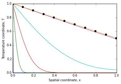
The result for the same system as above with $\mathrm{Nu}=N\mathrm{Nu}_{x}=1$ is:

$\hskip1in$

The analytical solution is given by:

$$T=T_h-\left(T_h-T_{\infty}\right)\frac{\mathrm{Nu}}{1+\mathrm{Nu}}\frac{x}{L}$$ $$\mathrm{Nu}=\frac{hL}{k}=\mathrm{Nu}_{x}\frac{L}{\Delta x}=N\mathrm{Nu}_{x}$$

Simulating a composite material

To simulate a composite material, we define an interface located at $x=x_b$ located at node $i=i_b$ where the region $1$ ($0\le x\lt x_b$) is characterized by $\alpha_1$ and region $2$ ($x_b\lt x\le L$) is characterized by $\alpha_2$. At the interface, there must be thermal equilibrium and thermal flux continuity:

$$T_{1}\left(x_{b},t\right)=T_{2}\left(x_{b},t\right)$$

$$-k_{1}\partial_{x}T_{1}\left(x_{b},t\right)=-k_{2}\partial_{x}T_{2}\left(x_{b},t\right)$$

where $i_b^-$ and $i_b^+$ are the nodes $i$ closest to the interface in region $1$ and $2$ respectively; i.e. $i_b^-=\mathrm{floor}(i_b)$ and $i_b^+=\mathrm{ceil}(i_b)$.

We discretize the equations:

$$\frac{\bar{T}_{i_{b}^{-},1}+\bar{T}_{i_{b}^{-}+\Delta x,1}}{2}=\frac{\bar{T}_{i_{b}^{+}-\Delta x,2}+\bar{T}_{i_{b}^{+},2}}{2}$$

$$-k_{1}\frac{\bar{T}_{i_{b}^{-}+\Delta x,1}-\bar{T}_{i_{b}^{-},1}}{\Delta x}=-k_{2}\frac{\bar{T}_{i_{b}^{+},2}-\bar{T}_{i_{b}^{+}-\Delta x,2}}{\Delta x}$$

and solve for the ghost nodes:

$$\bar{T}_{i_{b}^{-}+\Delta x,1}=\frac{\kappa-1}{\kappa+1}\bar{T}_{i_{b}^{-},1}+\frac{2}{\kappa+1}\bar{T}_{i_{b}^{+},2}$$

$$\bar{T}_{i_{b}^{+}-\Delta x,2}=\frac{2\kappa}{\kappa+1}\bar{T}_{i_{b}^{-},1}-\frac{\kappa-1}{\kappa+1}\bar{T}_{i_{b}^{+},2}$$

where $\kappa = k_1/k_2$.

The ODEs closest to the interface node are changed to:

$$\partial_{t}\bar{T}_{i_{b}^{-}}=\frac{\alpha_{1}}{\Delta x^{2}}\left[\bar{T}_{i_{b}^{-}-\Delta x}-\left(2-\frac{\kappa-1}{\kappa+1}\right)\bar{T}_{i_{b}^{-}}+\frac{2}{\kappa+1}\bar{T}_{i_{b}^{-}+\Delta x}\right]$$

$$\partial_{t}\bar{T}_{i_{b}^{+}}=\frac{\alpha_{2}}{\Delta x^{2}}\left[\frac{2\kappa}{\kappa+1}\bar{T}_{i_{b}^{+}-\Delta x}-\left(2+\frac{\kappa-1}{\kappa+1}\right)\bar{T}_{i_{b}^{+}}+\bar{T}_{i_{b}^{+}+\Delta x}\right]$$

which modifies the linear system to:

$$\partial_{t}\bar{\boldsymbol{T}}=\boldsymbol{\omega}\cdot\left(\boldsymbol{A}\cdot\bar{\boldsymbol{T}}+\boldsymbol{b}\right)$$

$$\boldsymbol{A}=\begin{bmatrix}-3 & 1\\ 1 & -2 & 1\\ & \ddots & \ddots & \ddots\\ & & 1 & -2 & 1\\ & & & 1 & -\left(2-\gamma\right) & \frac{2}{\kappa+1}\\ & & & & \frac{2\kappa}{\kappa+1} & -\left(2+\gamma\right) & 1\\ & & & & & 1 & -2 & 1\\ & & & & & & \ddots & \ddots & \ddots\\ & & & & & & & 1 & -2 & 1\\ & & & & & & & & 1 & -\left(2-\delta\right) \end{bmatrix}$$

$$\gamma=\frac{\kappa-1}{\kappa+1}\quad\delta=\frac{1-\frac{1}{2}\mathrm{Nu}_{x}}{1+\frac{1}{2}\mathrm{Nu}_{x}} $$

$$b=\begin{bmatrix}2T_{h}\\ \\ \\ \\ \\ \\ \\ \\ \\ \frac{\mathrm{Nu}_{x}}{1+\frac{1}{2}\mathrm{Nu}_{x}}T_{\infty} \end{bmatrix}\quad\boldsymbol{\omega}=\frac{1}{\Delta x^{2}}\begin{bmatrix}\alpha_{1}\\ & \ddots\\ & & \ddots\\ & & & \ddots\\ & & & & \alpha_{1}\\ & & & & & \alpha_{2}\\ & & & & & & \ddots\\ & & & & & & & \ddots\\ & & & & & & & & \ddots\\ & & & & & & & & & \alpha_{2} \end{bmatrix} $$

where I have defined a new matrix $\boldsymbol{\omega}$ which takes care of different values of $\alpha$ at different nodes.

To obtain the temperature at $x=x_b$, we have: $$T_{x_{b},1}=\frac{\bar{T}_{i_{b}^{-},1}+\bar{T}_{i_{b}^{-}+\Delta x,1}}{2}=\frac{\kappa}{\kappa+1}\bar{T}_{i_{b}^{-},1}+\frac{1}{\kappa+1}\bar{T}_{i_{b}^{+},2}$$

$$T_{x_{b},2}=\frac{\bar{T}_{i_{b}^{+}-\Delta x,2}+\bar{T}_{i_{b}^{+},2}}{2}=\frac{\kappa}{\kappa+1}\bar{T}_{i_{b}^{-},1}+\frac{1}{\kappa+1}\bar{T}_{i_{b}^{+},2} $$

which shows $T_{x_{b},1}=T_{x_{b},2}$ as imposed by the boundary condition at the interface.

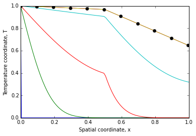
Solving this system, with similar parameters as above and $\alpha_1=k_1=10$ and $\alpha2=k_2=1$ yields this nice result:

$\hskip1in$

The analytical solution is given by:

$$T_{1}=T_{h}+\left(T_{\infty}-T_{h}\right)\frac{1}{\kappa}\frac{\Gamma\Pi}{1+\Pi}\frac{x}{L}$$

$$T_{2}=T_{h}+\left(T_{\infty}-T_{h}\right)\frac{1+\Gamma\Pi\frac{x}{L}}{1+\Pi}$$

$$\Gamma=\frac{\mathrm{Nu}}{1+\mathrm{Nu}}\quad\Pi=\frac{1}{\Gamma}\frac{L}{x_{b}}\frac{\kappa}{1-\kappa}$$

Python code:

The following Python code is used to generate the results.

import math
import numpy as np
import scipy.integrate as spi
import matplotlib.pyplot as plt

from __future__ import division, print_function

l, xb = 1, 0.5
a2, alpha = 1, 10 #alpha = a1/a2
k2, kappa = 1, 10 #kappa = k1/k2
Th, Tinf = 1, 0
Nu = 1 #= hL/k2
tp = l**2/a2

n = 100
dx = l/n
Nux = Nu/n

ib = n*xb/l-0.5
ibm = int(math.floor(ib))
ibp = int(math.ceil(ib))

A = np.zeros((n,n))
b = np.zeros((n,))
omega = np.zeros((n,n))

A[0,0], A[0,1], b[0], omega[0,0] = -3, 1, 2*Th, alpha*a2/dx**2
for i in xrange(1,ibm):
    A[i,i-1], A[i,i], A[i,i+1], omega[i,i] = 1, -2, 1, alpha*a2/dx**2
A[ibm,ibm-1], A[ibm,ibm], A[ibm,ibm+1], omega[ibm,ibm] = 1, -(2-(kappa-1)/(kappa+1)), 2/(kappa+1), alpha*a2/dx**2
A[ibp,ibp-1], A[ibp,ibp], A[ibp,ibp+1], omega[ibp,ibp] = 2*kappa/(kappa+1), -(2+(kappa-1)/(kappa+1)), 1, a2/dx**2
for i in xrange(ibp+1,n-1):
    A[i,i-1], A[i,i], A[i,i+1], omega[i,i] = 1, -2, 1, a2/dx**2
A[n-1,n-2], A[n-1,n-1], b[n-1], omega[n-1,n-1] = 1, -(2-(1-Nux/2)/(1+Nux/2)), Nux/(1+Nux/2)*Tinf, a2/dx**2

def diff_eq(T,t):
    return np.dot(omega, np.dot(A,T) + b)

i = np.linspace(0,n-1,n)
x = l/n*(i+1/2)
t = tp*np.logspace(-4,1,6)
T0 = Tinf*np.ones((n,))

sol = spi.odeint(diff_eq, T0, t)

## boundary condition at x=0
x = np.insert(x, 0, 0)
sol = np.insert(sol, 0, Th, axis=1)
## boundary condition at x=l
x = np.insert(x, n+1, l)
Tl = (Nux/2*Tinf + sol[:,-1])/(1+Nux/2)
sol = np.insert(sol, n+1, Tl, axis=1)

gamma = Nu/(1+Nu)
pi = l/xb/gamma*kappa/(1-kappa)
ana1 = Th+(Tinf-Th)*(gamma*pi/kappa*x/l)/(1+pi)
ana2 = Th+(Tinf-Th)*(1+gamma*pi*x/l)/(1+pi)
ana = np.append(ana1[x<xb],ana2[x>=xb])

plt.plot(x, np.transpose(sol), '-',
         x[::n//10], ana[::n//10], 'o')
plt.xlabel('Spatial coordinate, x')
plt.ylabel('Temperature coordinate, T')
plt.show()

Second order approximations on boundaries:

I want to quickly show that these approximations are indeed second-order accurate. To do this we take a Taylor expansion about the relevant boundary:

$$T\left(x_{b}+\frac{1}{2}\Delta x,t\right)=T\left(x_{b},t\right)+\partial_{x}T\left(x_{b}\right)\cdot\frac{1}{2}\Delta x+\frac{1}{2}\partial_{x}^{2}T\left(x_{b}\right)\cdot\left(\frac{1}{2}\Delta x\right)^{2}+O\left(\Delta x^{3}\right)$$

$$T\left(x_{b}-\frac{1}{2}\Delta x,t\right)=T\left(x_{b},t\right)-\partial_{x}T\left(x_{b}\right)\cdot\frac{1}{2}\Delta x+\frac{1}{2}\partial_{x}^{2}T\left(x_{b}\right)\cdot\left(\frac{1}{2}\Delta x\right)^{2}+O\left(\Delta x^{3}\right)$$

If we add these equations:

$$T\left(x_{b}+\frac{1}{2}\Delta x,t\right)+T\left(x_{b}-\frac{1}{2}\Delta x,t\right)=2T\left(x_{b},t\right)+O\left(\Delta x^{2}\right)$$

and rearrange we get:

$$T\left(x_{b},t\right)=\frac{T\left(x_{b}+\frac{1}{2}\Delta x,t\right)+T\left(x_{b}-\frac{1}{2}\Delta x,t\right)}{2}+O\left(\Delta x^{2}\right)$$

which is our approximation for the temperature at a boundary shown to be indeed second-order in $\Delta x$.

If we subtract the two Taylor expansion: $$T\left(x_{b}+\frac{1}{2}\Delta x,t\right)-T\left(x_{b}-\frac{1}{2}\Delta x,t\right)=\partial_{x}T\left(x_{b}\right)\Delta x+O\left(\Delta x^{3}\right)$$

and rearrange, we get: $$\partial_{x}T\left(x_{b}\right)=\frac{T\left(x_{b}+\frac{1}{2}\Delta x,t\right)-T\left(x_{b}-\frac{1}{2}\Delta x,t\right)}{\Delta x}+O\left(\Delta x^{2}\right)$$

which is the approximation for the temperature gradient at a boundary, again shown to be second-order accurate in $\Delta x$.