TL;DR: Real life equations are created by carefully observing relationships between different quantities, making simplification assumptions, and then abstracting them into a mathematical form.
I've posted below a few examples of how to derive DE's from "real life" examples for a range of sciences. Hopefully, they will give a glimpse of the process.
Example of Predator - Prey equation 1
The primary prey for the Canadian lynx is the snowshoe hare. We will denote the population of hares by $H(t)$ and the population of lynx by L(t), where t is the time measured in years. Assuming that :
- If no lynx are present, we will assume that the hares reproduce at a rate proportional to their population and are not affected by overcrowding. That is, the hare population will grow exponentially,
$$\frac{dH(t)}{dt}=aH(t)$$
where: a is a constant.
- Since the lynx prey on the hares, we can argue that the rate at which the hares are consumed by the lynx is proportional to the rate at which the hares and lynx interact. Therefore some hares will be preyed upon and removed from the population. Thus, the equation that predicts the rate of change of the hare population becomes:
$$\frac{dH(t)}{dt}=aH(t)−bH(t) L(t)$$
where: a, b are constants for reproduction and interaction respectively
We are thinking of H(t) L(t) as the number of possible interactions between the lynx and the hare populations.
- If there is no food, the lynx population will decline at a rate proportional to itself,
$$\frac{dL(t)}{dt}=\delta L(t)$$
where: δ is a constant for declining population (old age/starvation etc).
- The lynx receive benefit from the hare population. The rate at which lynx are born is proportional to the number of hares that are eaten, and this is proportional to the rate at which the hares and lynx interact. Consequently, the growth rate of the lynx population can be described by:
$$\frac{dL(t)}{dt}=c H(t)L(t)−\delta L(t)$$
where c, δ are constants.
We now have a system of differential equations that describe how the two populations interact,
$$\begin{cases}
\frac{dH(t)}{dt}=aH(t)−bH(t) L(t)\\
\frac{dL(t)}{dt}=c H(t)L(t)−\delta L(t)
\end{cases}
$$
if you use $x(t)=H(t)$,$y(t)=L(t)$, the above set of equation can be rewritten in a more conventional form:
$$\begin{cases}
\dot{x}=a\cdot x−b\cdot x\cdot y\\
\dot{y}=c \cdot x\cdot y−\delta \cdot y
\end{cases} \rightarrow
\begin{cases}
\dot{x}= x \cdot (a−b\cdot y) \\
\dot{y}= (c \cdot x−\delta) \cdot y
\end{cases}
$$
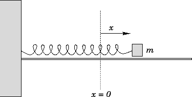
Mechanical Harmonic Oscillator
Another typical example is the harmonic oscillator. Below is

Newtons second law of motion states that the acceleration of an object is directly proportional to the sum of all forces (net force) and inversely proportional to the mass.
$$\sum F = m a $$
where:
- m : mass
- $a = \ddot{x}$: the acceleration along the horizontal axis.
- $\sum F$ is the net force.
The force only force applied in this example is the spring force. The spring force is proportional to the displacement x, according to Hooke's Law. Therefore:
$$F_{spring} = -k\cdot x$$
Therefore, because $\sum F=-k x$, Newton's Law becomes $-kx = m a $, or (if you replace $a = \ddot{x}$) it more recognizable form for DE:
$$- kx = m \ddot{x}$$
or
$$m \ddot{x} + kx =0$$
RLC circuit
you can find a nice derivation for the RLC electrical circuit here
Starting from Kirchoff's law, using Ohm law and other basic relationships to derive:
$$L \frac{d^2 q}{dt^2}+ R\frac{d q}{dt} + \frac{1}{C} q(t) = V_0\sin(\omega t)$$
